|
This page was designed for an undergraduate course at Davidson College. Background: Microarrays, Expression, Hierarchical clustering
|
I. Microarrays:
Traditional genetics experiments manipulated single genes or
monitored the effects of a single gene in different experimental
conditions. Although these are valid methods of gathering data about
genes, they unearth very little information about other genes or how single genes may
interact with the collective gene product in a living organism. The
microarray is an exceptionally powerful genomic tool, capable of examining
thousands of genes simultaneously. By examining microarray data,
researchers can infer the relationships between genes and thus gain a better
understanding of how genes interact within an organism.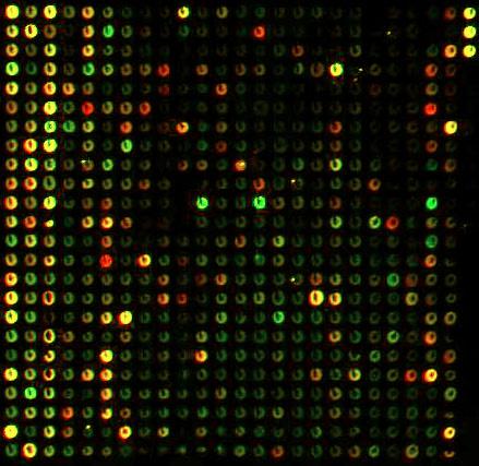
Physically, microarrays (also known as gene chips, DNA arrays, or gene arrays) are small chips (often made of glass) with thousands of small embedded wells or spots. Each spot represents one gene, and all of the genes in the genome may be represented on the same chip. Each spot contains fluorescent dye chemically bonded to the DNA or RNA at that spot. The relative levels of the dye can be optically analyzed and used to infer the relative levels of expression of each gene. Thus, a single microarray can simultaneously represent the expression of an entire genome of an organism, and because the genes are lined up into ordered arrays, each gene can be individually identified.
How do you get from gene expression within a cell to a microarray with colored dyes representing each gene? There are several steps in the microarray process (for a more complete description visit www.gene-chips.com):
-
Synthesize the Probes. First a microarray is prepared either specifically for the genes of interest, or for all of the genes in the organism of interest's genome. This is done by synthesizing a complementary probe to the mRNA for each gene. The most common technique for doing this is to use robotic systems to individually synthesize thousands of probes in situ, with one spot containing thousands of oligonucleotide probes for a single gene.
-
Acquire the mRNA. The population of cells you wish to analyze must be treated such that only the mRNA, representing all of the expressed genes in those cells, is extracted.
-
Label the mRNA. The mRNA from the cells is then labeled with a fluorescent dye. For the present discussion, assume that red represents the control mRNA, and green represents the mRNA of the experimental condition.
-
Hybridization. Both the experimental and the control mRNA are simultaneously washed over the microarray. Whenever the probes on a given spot interact with a complementary mRNA strand the two will hybridize, thus binding the mRNA to the microarray. After a certain period of time the remaining solution is discarded and the microarray is gently rinsed.
-
Fluorescence Analysis. The microarray is then scanned optically and the ratios of red to green are computed. Since red represents the control mRNA and green represents the experimental mRNA, the colors on each spot will reflect how the expression of each gene was changed by the manipulation of the experimental condition. Often a new image of the microarray is formed almost exactly the same as the original, with the exception that now green means a reduction in expression, and red means an increase in expression.
-
Data Analysis. The ratios of red:green are next analyzed mathematically for relationships among the genes. This step is where hierarchical clustering is useful.
The microarray data used on this student web page were produced by Gasch et al. (2000) at Stanford University using the yeast Sacchromyces cerevisiae. These data are publicly available. Stanford is well-known in the field of yeast biology for their extensive genomic research and database maintenance. Gasch et al.'s experiments examined how the expression of all proteins in the yeast genome change when the yeast are exposed to different environments of high "stress." Our clustering interface on this website allows you to choose to analyze the data from four of these stress condition experiments, although Gasch et al. produced data on several other experimental conditions. The four readily available on this website are two different heat shock experiments, hydrogen peroxide stress, and nitrogen depletion. If you are particularly interested in the original data set, you may wish to examine it more in depth here.
It's important to remember that microarrays don't provide any spatial information. In other words, even if two genes are induced in the same experimental condition, one gene could be a cell membrane protein and the other could be a transcription factor that regulates Golgi transport (i.e., relatively un-related). Perhaps the two are related in the big cellular picture and perhaps not: the caveat here is that the numbers provided by expression data cannot tell the complete story. Empirical studies that unequivocally define the relationships between genes and how that relates to intracellular location or organelle localization remain extremely important.
II. Gene Expression: Determining Repression or Induction
The ratios of fluorescence on a microarray must be optically analyzed to determine whether there has been repression or induction. The fluorescence of both colors (red and green) at each spot is quantified by an image scanner. Recall that red represents the control mRNA, and green represents the experimental mRNA. Each spot is then given a ratio of green:red, which tells us whether that particular gene was produced in greater quantities (induced) or produced in smaller quantities (repressed) in comparison to the baseline amount of expression. This expression ratio is subsequently divided to give a decimal value and then converted to a logarithmic (base 2) scale.
![]()
A logarithmic scale is commonly used when computing expression data. Logarithmic scales make it very easy to conceptualize repression versus induction. For example, if the experimental expression is greater than the control expression the ratio will be greater than one, and thus the final number after logarithmic transformation will be positive. If the experimental expression is less than controls, however, the final number will be negative. Note also that whenever control and experimental expression is 1:1, the final result will be 0.
The resulting data can be converted into images in order to quickly assess repression or induction visually. The scale is confusingly labeled in green and red as well, so it is very important to remember that these colors represent the changes in expression and not the initial fluorescence from mRNA hybridization. A typical scale would look something like this, where a black spot on the array would indicate that equal amounts of red and green fluorescence were observed on the original spot, thereby giving an equal expression ratio of 1:1, and subsequently a logarithmic value of 0.
![]()
Although the process is straight-forward in theory, the actual practice of this transition from fluorescence to numerical values can be challenging. One of the first problems researchers have to deal with is "gridding", or figuring out how to tell the computer where to look for fluorescence within the spot on the grid. Within each spot, mRNAs hybridize to the oligonucleotides completely randomly and with different intensities in different areas of the spot. Programming a computer to recognize and distinguish between each spot and "accept" this randomness while accurately and thoroughly measuring fluorescence has proven to be quite difficult.
Additionally, image processing and ratio quantification have been stumbling blocks in the calculation of expression ratios. Essentially, scientists are still determining how different concentrations of mRNA, fluorescent tags, and oligonucleotide density affect the accuracy and standardization of ratio determination. One of Michael Eisen's programs, ScanAlyze is one of the best (and free) programs currently in the industry.
III. Hierarchical Clustering:
Once researchers have determined the amount of repression or induction for each gene represented in the microarray the data must be "sorted" computationally using algorithms. One such algorithm, hierarchical clustering, is described below. First, however, consider the potential biological information that is sought when analyzing microarray data. By joining or "clustering" similarly expressed genes we can identify groups of genes that are "turned on/off" in response to the same environmental factors. This sort of information is particularly useful in beginning to understand functional pathways and how gene products interact. In particular, a few biologists such as Eric Davidson have had tremendous success deducing regulational control of genes and have found hard-wired, yet dynamic developmental pathways using microarrays and new computational programming.
Hierarchical clustering requires two main steps that are repeated in order to find the genes that are most similar. As an overview, hierarchical clustering finds the pair of genes that are most similar, joins them together, and then identifies the next most similar pair of genes. This process continues until all of the genes are joined into one giant cluster.
How do you assess the similarity of genes' expression patterns? One way to do so is the Pearson correlation coefficient, symbolized by a lowercase r or the Greek letter rho. A Pearson correlation coefficient indicates the relationship between two ordered sets of numbers (in this case, gene expression data for several different conditions). It indicates both how the two sets are related and the strength of that relationship. For example, if gene A increases over time and gene B decreases proportionally, their correlation value will be -1.0 because they are perfectly divergent. If the two sets were not perfectly divergent, but still diverged, the correlation would remain negative, but would be greater than -1.0. In contrast, if genes A and B increase proportionally over time, then their correlation will be 1.0. If genes A and B have absolutely no relationship to each other whatsoever, their correlation will be 0. The Pearson correlation coefficient is sensitive to not only direction of change (increasing or decreasing), but also to magnitude of change (Did gene A increase 2-fold while gene B increased only 1-fold?). A correlation coefficient is always between -1 and 1.
a) Computing a Pearson Correlation Coefficient
The Pearson correlation coefficient can be computed a number
of ways. First let X be the set of data points
![]() for gene X, and let Y be the set of data points
for gene X, and let Y be the set of data points
![]() for gene Y. The easiest form to represent symbolically is
for gene Y. The easiest form to represent symbolically is
![]()
where
the numerator is the sum of the product of the z-scores (normalized values) at
each respective
![]() pair, and N represents the total number of pairs. In
practice, however, the correlation can be computed using the formula
pair, and N represents the total number of pairs. In
practice, however, the correlation can be computed using the formula

where Sxx and Syy represent the sum of squares, and Sxy represents a sum of products. Symbolically,
![]() ,
,
![]() ,
,
![]() .
.
Thus, the final, computational form, of the Pearson correlation coefficient becomes
To return to the context of hierarchical clustering, a Pearson correlation coefficient must be computed for every possible gene comparison. When clustering an entire genome of 6,000 or more genes this can mean a considerable number of comparisons must be performed, yet the results can provide valuable generalizations about the genes' relationships.
b) Forming Clusters and Pseudo-Genes
Once you have a table of correlation values between each of the genes being clustered you must select the gene pair that has the highest correlation value. These two genes are the first cluster.
The
next step is to merge the two clustered genes into a new
"pseudo-gene". The new pseudo-gene will contain the same
number of data points, but each point will now be the arithmetic mean of the
two original data points
![]() .
The two original genes that were merged are removed from the table of
correlation values, and new correlations are found between the new pseudo-gene
and all of the remaining genes in the table. Next, find the highest
remaining correlation value in the table and join that pair of genes into a
new pseudo-gene. This process continues until all that remains is a
single pseudo-gene containing the arithmetic mean of all the original genes at
each data point.
.
The two original genes that were merged are removed from the table of
correlation values, and new correlations are found between the new pseudo-gene
and all of the remaining genes in the table. Next, find the highest
remaining correlation value in the table and join that pair of genes into a
new pseudo-gene. This process continues until all that remains is a
single pseudo-gene containing the arithmetic mean of all the original genes at
each data point.
When clustering an original gene with a previously formed pseudo-gene the new pseudo-gene that is formed must be an arithmetic mean of all the genes' data that it contains, not a simple average between the pseudo-gene's data and the original gene's data. In other words, each gene carries equal weight when computing the pseudo-gene's data, regardless of the order in which the genes were originally clustered.
Notice that by selecting only the maximally correlated genes to be joined together at each step some possible relationships will not be indicated by the final clustering order. For example, if gene A is perfectly negatively correlated with gene B (r = -1.00) genes A and B will never cluster together even though they are obviously related. Such "inverse" relationships will not be detected using hierarchical clustering.
c) Thresholds and "Cutting the Tree"
By retracing the order in which the genes were progressively joined into clusters and by knowing the correlation value of each step, you can map out which genes are related to each other closely and which genes are related only distantly. This is best represented graphically, as shown by the following hypothetical diagram.
A threshold can be set at any value between -1 and 1 where any genes paired with correlations greater than that threshold can be considered a cluster, and any genes or clusters with correlations less than that threshold are not. This is known as "cutting the tree". By setting a threshold value, you are essentially saying, "All genes must have a correlation greater than my threshold in order to consider them a cluster." For example, if the threshold were to be set at 0.75 in the above example, there would only be one cluster (genes E and G) and all of the rest of the genes would be unclustered. However, if the threshold were set at 0.50, there would be two clusters and one free gene (Cluster 1: ADFBC; Cluster 2: EG; free gene: H).
The order of clustering events for the above case (with hypothetical correlation values) would be 1) E & G at r=0.78, 2) A & D at r=0.70, 3) F & B at r=0.65, 4) AD & FB at r=0.61, 5) ADFB & C at r=0.59, 6) EG & H at r=0.29, and 7) ADFBC & EGH at r=-0.55.
Clustered genes can then be grouped together and the original data can be graphed to visually depict the degree of similarity within the cluster.
Software that can be downloaded to perform your own clustering analysis offline: Michael Eisen's Cluster program.
References:
Gasch et al. 2000. Genomic expression programs in the response of yeast cells to environmental changes. Mol. Bio. Cell. 11(12) 4241-4257.
|
E-mail the authors: amhartman@davidson.edu, sojohnson@davidson.edu, jekawwass@davidson.edu Go to Davidson College: Biology Department or Math Department
This page was designed for an undergraduate course, Computational Biology, at Davidson College.
|